Why does CUBIC take us back to TCP congestion control?

TCP Congestion Control: basic outline and TCP CUBIC algorithm

TCP congestion control is a fundamental part of this protocol and over the years has undergone a process of constant improvement through the generation of different versions, such as TCP Tahoe, Reno, Vegas, and so on.

The case of the TCP CUBIC version, which has been the default congestion control applied by Linux/Unix systems.

TCP CUBIC becomes even more interesting since Microsoft has decided that this version is a fundamental part of products such as Windows 10 and Windows Server 2019, as read in this document on the news of Windows Server 2019 and in this on Windows 10.

Having the same distribution in Linux and Windows environments has led network administrators to review the idea behind the congestion control posed by TCP and what TCP CUBIC implies.

Let’s start by reviewing the fundamental idea of TCP congestion control.

Window management as a basis for congestion control

TCP introduces the concept of “windows” to establish traffic flow control and manage connections between two devices: a sender and a receiver.

Thus, the basic implementation is known as the receive window, in which, per connection, a window size is set that represents the amount of packets that the sender can send to the receiver without waiting for recognition packets (ACK packets).

However, the slider protocol manages the connection based on the buffer capacities of the receiving equipment, but it does not recognize the congestion problems associated with the network.

To adjust the transmission depending on the level of congestion, TCP introduces another window. This is the congestion window or cwnd to regulate the number of packets sent based on TCP’s perception of the congestion.

But how does TCP perceive congestion on the network and what does it do accordingly?

The basic idea is as follows:

1. If there are lost packets, it is assumed that there is congestion on the network, and packet loss is evaluated on the basis of received and not received acknowledgement packets.
2. If congestion is determined to exist, the congestion window is modified in such a way that the sender slows down the sending of its packages.
3. If no congestion is determined, the congestion window will be modified so that the sender can send more packets.

On this basic procedure we find multiple algorithms that implement it.

Algorithms propose things like how many not received ACK packets involve congestion, how much to decrease or increase the cwnd window, how to calculate the transfer rate from the congestion window, etc.

Then we suggest you to review the evolution of these algorithms in order to have a clear understanding of the scope of those currently in use.

Evolution of congestion control algorithms

The evolution of TCP congestion control began in the mid-1980s.

Up to that point, streaming control based on sliding windows had worked quite well, but with the popularization of the Internet, congestion became a problem.

Between 1986 and 1988, Van Jacobson proposed the basic congestion control scheme and developed the first implementation protocol, known as TCP Tahoe.

The transmission ratio should take into account the value of the reception and congestion windows, leaving the transmitter restricted to a transmission ratio whose minimum value is rwnd and its maximum is cwnd.

In 1990 with TCP Reno the application of the AIMD algorithm (additive increase / multiplicative decrease) was introduced:

1. The transmission rate will gradually increase until some packet loss occurs.
2. The increase will be made by linearly increasing the congestion window, i.e. by adding a value.
3. If congestion is inferred, the transmission ratio will be decreased, but in this case a decrease will be made by multiplying by a value.

After TCP Reno other algorithms and versions of TCP appeared that tried to take the precepts of congestion control and refine it, experiencing a great diversification of versions and scopes.

Thus we have that TCP Vegas raises attention to the values of delay to infer congestion or the case of ECN (Explicit Congestion Notification) that introduces the possibility that the routers of the network notify congestion conditions to the transmitting equipment.

It has also promoted the development of a good number of mechanisms that allow the implementation of AIMD, such as Slow Start, Fast Retransmission, Fast recovery, Adaptive timeout or ACK clocking.

In any case, it is interesting to clarify the situation we had until recently.

The Linux world had opted for TCP CUBIC, which is an heir to TCP Reno and BIC TCP, so it relies on packet loss rather than on delay values to determine congestion.

While the Windows world used an algorithm called TCP Compound, which comes from TCP Fast, which in turn is heir to TCP Vegas, so they rely on delays to infer congestion.

As we mentioned at the beginning of this article, this situation changed when Microsoft decided to introduce TCP CUBIC in its new products.

TCP CUBIC

TCP CUBIC is a congestion control algorithm that arises with the idea of taking advantage of the fact that today’s communications links tend to have increasingly higher bandwidth levels.

In a network composed of wide bandwidth links, a congestion control algorithm that slowly increases the transmission rate may end up wasting the capacity of the links.

The intention is to have an algorithm that works with congestion windows whose incremental processes are more aggressive, but are restricted from overloading the network.

In order to achieve this, it is proposed that the scheme for increasing and decreasing the transmission ratio be established according to a cubic function. Let’s see the next figure:

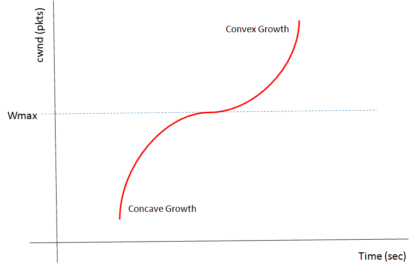
Description: Cubic function that regulates the congestion window according to the Cubic algorithm
From: IEEE Xplore Digital Library: https://ieeexplore.ieee.org/document/8368259

The procedure followed by the algorithm is:

1. At the time of experiencing congestion event the window size for that instant will be recorded as Wmax or the maximum window size.
2. The Wmax value will be set as the inflection point of the cubic function that will govern the growth of the congestion window.
3. The transmission will then be restarted with a smaller window value and, if no congestion is experienced, this value will increase according to the concave portion of the cubic function.
4. As the window approaches Wmax the increments will slow down.
5. Once the tipping point has been reached, i.e. Wmax, the value of the window will continue to increase discreetly.
6. Finally, if the network is still not experiencing any congestion, the window size will continue to increase according to the convex portion of the function.

As we can see, CUBIC implements schemes of large increments at first, which decrease around the window size that caused the last congestion, and then continue to increase with large increments.

If you want to learn more about the technical details of the CUBIC algorithm, you can read the following work:
https://www.cs.princeton.edu/courses/archive/fall16/cos561/papers/Cubic08.pdf

Congestion control and monitoring tools

An interesting point of congestion control provided by TCP is that these are processes with the following characteristics:

1. These processes run only in the emitting equipment.
2. They don’t generate traffic.
3. They promote an equitable distribution of the transmission capacity of the network. As each device decides on its transmission capacity, taking into account only the behaviour of the network it observes, no emitting device is favoured or harmed under any circumstances.

However, it is easy to understand that it is not fair to compare the capabilities of TCP’s congestion control algorithms with the capabilities of a monitoring tool, because we are moving in two completely different universes.

However, we propose you to think about the scope of a general purpose monitoring tool like Pandora FMS from the angle of these algorithms.

These are the following points:

1. The object of study of a monitoring tool is much broader: a monitoring tool must consider all the protocols present on the platform, not just TCP.
2. The idea of a monitoring tool is to include under its scheme all the components, always offering a global vision of the platform.
3. The mechanisms used by a monitoring tool, such as those associated with network management such as SNMP or with traffic flow control such as NetFlow, are protocols that involve sending packets associated with their functions. Now, of course, the monitoring tools aim to establish a scheme that interferes just enough with the overall performance of the platform.
4. The root cause of congestion: The approach achieved by the monitoring tools aims to get to the root cause of congestion. Perhaps the cause of a state of congestion is in the wrong configuration of a routing protocol, which is not going to be corrected by the emitting equipment modifying its transmission capacity.
5. To conclude, we must say that one objective of the monitoring tools is to generate information that allows predicting a congestion situation before it appears.

Have a look at this interesting article on bandwidth monitoring.

In addition, if you do not yet have a monitoring tool for the platform, you should know that you have come to the right place. In fact, if you have more than 100 devices we suggest you evaluate Pandora FMS Enterprise.

And if you have a reduced number of devices we recommend you to download the Pandora FMS Open Source version.